Dynamic Ensembles: Comparing Several Approaches
This notebook explores how to combine nixtla’s neuralforecast models using several ensemble approaches.
Loading M3’s monthly dataset
Preparing and running cross-validation with 7 neural networks
Fitting several combination rules using out-of-sample data from cross-validation
Getting forecasts and combining them
Evaluating all models
[1]:
import warnings

warnings.filterwarnings("ignore")
If necessary, install the package using pip:
[2]:
# !pip install metaforecast=='0.1.3'
1. Data preparation
Let’s start by loading the dataset. This tutorial uses the M3 monthly dataset available on datasetsforecast.
We also set the forecasting horizon and input size (number of lags) to 12.
[3]:
import pandas as pd

from datasetsforecast.m3 import M3

horizon = 12
n_lags = 12

df, *_ = M3.load('.',group='Monthly')
Split the dataset into training and testing sets:
[4]:
df_by_unq = df.groupby('unique_id')

train_l, test_l = [], []
for g, df_ in df_by_unq:
    df_ = df_.sort_values('ds')

    train_df_g = df_.head(-horizon)
    test_df_g = df_.tail(horizon)

    train_l.append(train_df_g)
    test_l.append(test_df_g)

train_df = pd.concat(train_l).reset_index(drop=True)
test_df = pd.concat(test_l).reset_index(drop=True)

train_df.query('unique_id=="M1000"').tail()
[4]:
| unique_id | ds | y | |
|---|---|---|---|
| 286 | M1000 | 1992-10-31 | 4563.4 |
| 287 | M1000 | 1992-11-30 | 4551.8 |
| 288 | M1000 | 1992-12-31 | 4577.4 |
| 289 | M1000 | 1993-01-31 | 4592.4 |
| 290 | M1000 | 1993-02-28 | 4632.2 |
[5]:
test_df.query('unique_id=="M1000"').head()
[5]:
| unique_id | ds | y | |
|---|---|---|---|
| 36 | M1000 | 1993-03-31 | 4625.6 |
| 37 | M1000 | 1993-04-30 | 4668.2 |
| 38 | M1000 | 1993-05-31 | 4598.0 |
| 39 | M1000 | 1993-06-30 | 4619.4 |
| 40 | M1000 | 1993-07-31 | 4640.4 |
2. Model setup and cross-validation
Let’s start by setting up the ensemble members: 7 neural networks based on neuralforecast.
We carry out a cross-validation procedure to get out-of-sample forecasts that will be used to fit the combination rule
[ ]:
from neuralforecast import NeuralForecast
from neuralforecast.models import (NHITS,
                                   LSTM,
                                   GRU,
                                   NBEATS,
                                   MLP,
                                   TiDE)

CONFIG = {
    'input_size': n_lags,
    'h': horizon,
    'accelerator': 'cpu',
    'max_steps':1000,
}

models = [
    NBEATS(**CONFIG, stack_types=3*["identity"]),
    NHITS(**CONFIG),
    MLP( **CONFIG),
    MLP(num_layers=3, **CONFIG),
    LSTM(**CONFIG),
    GRU(**CONFIG),
    TiDE( **CONFIG),
]


nf = NeuralForecast(models=models, freq='M')
[ ]:
%%capture

# should try nf.predict_insample
n_windows = train_df['unique_id'].value_counts().min() - n_lags - horizon
n_windows = int(n_windows // 2)

fcst_cv = nf.cross_validation(df=train_df, n_windows=n_windows, step_size=1)
fcst_cv = fcst_cv.reset_index()
fcst_cv = fcst_cv.groupby(['unique_id', 'cutoff']).head(1).drop(columns='cutoff')
[8]:
fcst_cv.head()
[8]:
| unique_id | ds | NBEATS | NHITS | MLP | MLP1 | LSTM | GRU | TiDE | y | |
|---|---|---|---|---|---|---|---|---|---|---|
| 0 | M1 | 1992-07-31 | 4270.607422 | 4316.121094 | 3988.292969 | 4269.679199 | 3331.872803 | 3312.583252 | 4209.511719 | 5880.0 |
| 12 | M1 | 1992-08-31 | 5383.976562 | 5088.954102 | 4664.032227 | 4608.907227 | 3408.262695 | 3532.260254 | 4589.873047 | 1680.0 |
| 24 | M1 | 1992-09-30 | 3962.103271 | 3926.756348 | 3292.554443 | 3432.223633 | 3158.096924 | 3155.144531 | 6003.843750 | 6720.0 |
| 36 | M1 | 1992-10-31 | 3850.518799 | 3936.579346 | 4416.983398 | 4314.682617 | 2995.153809 | 3089.166016 | 4937.783691 | 2040.0 |
| 48 | M1 | 1992-11-30 | 4311.153320 | 4394.302734 | 3661.406250 | 3534.437988 | 3103.114746 | 3088.328125 | 3061.584473 | 6480.0 |
3. Ensemble combination rule
In this example, we’ll compare several dynamic ensembles
[9]:
from metaforecast.ensembles import (MLpol, MLewa, ADE, LossOnTrain, BestOnTrain, EqAverage, Windowing)
[10]:
TRIM_R = 0.8

combiners = {
    'ADE': ADE(freq='M', meta_lags=list(range(1, 4)), trim_ratio=TRIM_R, trim_by_uid=False),
    'MLpol': MLpol(loss_type='square', gradient=True, trim_ratio=TRIM_R, weight_by_uid=False),
    'MLewa': MLewa(loss_type='square', gradient=True, trim_ratio=TRIM_R, weight_by_uid=False),
    'LossOnTrain': LossOnTrain(trim_ratio=TRIM_R, weight_by_uid=False),
    'BestOnTrain': BestOnTrain(select_by_uid=False),
    'EqAverage': EqAverage(select_by_uid=False, trim_ratio=TRIM_R),
    'Windowing': Windowing(freq='M', trim_ratio=TRIM_R, select_best=False, weight_by_uid=False),
    'BLAST': Windowing(freq='M', trim_ratio=TRIM_R, select_best=True, weight_by_uid=False),
}
[11]:
for k in combiners:
    print(f'Fitting {k}')
    combiners[k].fit(fcst_cv)
Fitting ADE
Fitting MLpol
Fitting MLewa
Fitting LossOnTrain
Fitting BestOnTrain
Fitting EqAverage
Fitting Windowing
Fitting BLAST
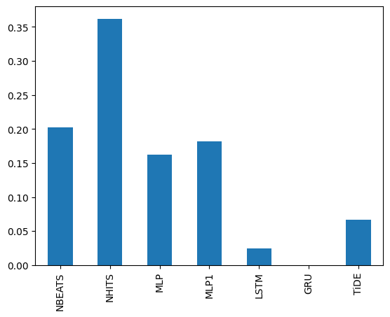
Let’s look at the weights of different combiners
[12]:
combiners['MLpol'].uid_coefficient['M1000'].plot.bar()
[12]:
<Axes: >
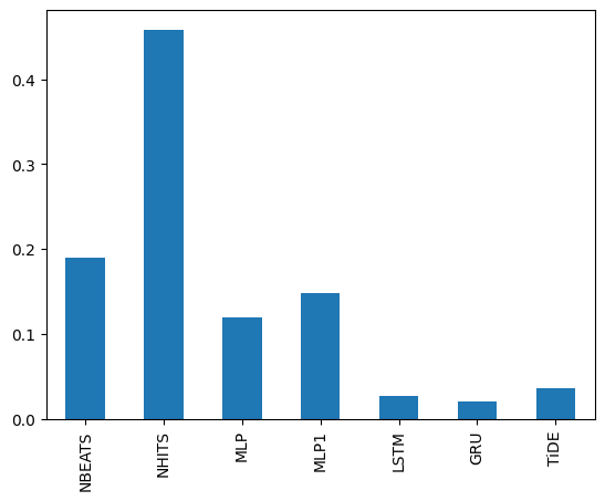
[13]:
combiners['MLewa'].uid_coefficient['M1000'].plot.bar()
[13]:
<Axes: >
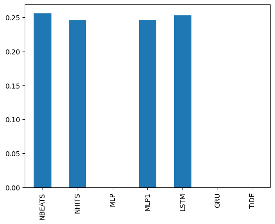
[14]:
combiners['Windowing'].weights.loc['M1000',:].plot.bar()
[14]:
<Axes: >
Then, we refit the neural networks are get the test forecasts
[ ]:
%%capture

nf.fit(df=train_df)
[ ]:
%%capture

fcst = nf.predict(step_size=1)
[17]:
fcst.query('unique_id=="M1"')
[17]:
| ds | NBEATS | NHITS | MLP | MLP1 | LSTM | GRU | TiDE | |
|---|---|---|---|---|---|---|---|---|
| unique_id | ||||||||
| M1 | 1994-09-30 | 2820.708008 | 2837.058838 | 2383.298828 | 2454.077393 | 2507.238525 | 2390.672607 | 2070.891602 |
| M1 | 1994-10-31 | 2353.479248 | 2515.124512 | 2158.801270 | 2129.693848 | 2583.255859 | 2305.683838 | 2451.634033 |
| M1 | 1994-11-30 | 2303.218750 | 2391.572754 | 2291.510254 | 2139.453857 | 2939.735107 | 2787.014160 | 1721.748047 |
| M1 | 1994-12-31 | 2779.379883 | 2526.065918 | 2591.097412 | 2590.750244 | 2814.711182 | 2776.601318 | 2240.189941 |
| M1 | 1995-01-31 | 2188.668457 | 2063.863525 | 2234.466553 | 1887.351929 | 2838.986328 | 2785.913818 | 1796.146118 |
| M1 | 1995-02-28 | 1911.853271 | 2175.461670 | 1985.965088 | 1816.956787 | 2691.198242 | 2710.279541 | 2631.498779 |
| M1 | 1995-03-31 | 2451.522461 | 2249.096436 | 2160.844971 | 1911.716309 | 2619.605469 | 2653.789551 | 1920.423096 |
| M1 | 1995-04-30 | 1735.337402 | 1839.155762 | 1614.420044 | 1335.228027 | 2504.666992 | 2538.148926 | 2000.088135 |
| M1 | 1995-05-31 | 1939.377686 | 2237.283691 | 2295.252930 | 2200.254150 | 2474.093994 | 2538.217285 | 3073.768555 |
| M1 | 1995-06-30 | 1589.561279 | 1889.871582 | 2036.288086 | 1789.682861 | 2385.954834 | 2385.965332 | 1627.879883 |
| M1 | 1995-07-31 | 2011.243408 | 2133.244385 | 1954.133423 | 1680.693481 | 2248.914551 | 2293.520508 | 1596.402466 |
| M1 | 1995-08-31 | 2416.882568 | 2366.746582 | 2237.609131 | 2308.385254 | 2482.302979 | 2661.940918 | 1933.988281 |
[18]:
ensemble_fcst = {}
for k in combiners:
    print(k)
    if k == 'ADE':
        # need to make sure unique_id is in columns
        fc = combiners[k].predict(fcst.reset_index(), train=train_df, h=horizon)
    else:
        fc = combiners[k].predict(fcst.reset_index())

    ensemble_fcst[k] = fc

ensemble_fcst_df = pd.DataFrame(ensemble_fcst)
ADE
MLpol
MLewa
LossOnTrain
BestOnTrain
EqAverage
Windowing
BLAST
[19]:
ensemble_fcst_df
[19]:
| ADE | MLpol | MLewa | LossOnTrain | BestOnTrain | EqAverage | Windowing | BLAST | |
|---|---|---|---|---|---|---|---|---|
| 0 | 2734.990919 | 2633.876117 | 2687.956142 | 2647.597933 | 2820.708008 | 2600.476318 | 2609.517685 | 2820.708008 |
| 1 | 2413.129298 | 2346.027112 | 2375.503276 | 2416.961861 | 2353.479248 | 2348.070947 | 2372.301306 | 2353.479248 |
| 2 | 2368.810476 | 2263.482370 | 2296.720479 | 2512.772930 | 2303.218750 | 2413.098145 | 2457.888033 | 2303.218750 |
| 3 | 2615.789141 | 2581.755320 | 2583.917473 | 2726.531104 | 2779.379883 | 2660.400928 | 2688.874069 | 2779.379883 |
| 4 | 2119.322474 | 2066.855810 | 2072.368257 | 2353.839662 | 2188.668457 | 2242.667358 | 2297.588398 | 2188.668457 |
| ... | ... | ... | ... | ... | ... | ... | ... | ... |
| 17131 | 5235.239195 | 5263.440157 | 5260.213604 | 5228.020998 | 5255.608398 | 5242.863867 | 5228.022853 | 5255.608398 |
| 17132 | 5236.594895 | 5274.892725 | 5272.110740 | 5228.778586 | 5260.446777 | 5251.575293 | 5228.879529 | 5260.446777 |
| 17133 | 5233.346570 | 5275.373552 | 5271.142153 | 5224.094460 | 5230.098633 | 5253.171680 | 5223.840454 | 5230.098633 |
| 17134 | 5247.344425 | 5305.818907 | 5300.775081 | 5238.732074 | 5271.788086 | 5278.508789 | 5238.902449 | 5271.788086 |
| 17135 | 5254.623441 | 5304.463775 | 5299.146796 | 5242.637530 | 5259.853516 | 5277.595410 | 5242.359317 | 5259.853516 |
17136 rows × 8 columns
[20]:
fcst_all = pd.concat([fcst.reset_index(),ensemble_fcst_df],axis=1)

fcst_all.head()
[20]:
| unique_id | ds | NBEATS | NHITS | MLP | MLP1 | LSTM | GRU | TiDE | ADE | MLpol | MLewa | LossOnTrain | BestOnTrain | EqAverage | Windowing | BLAST | |
|---|---|---|---|---|---|---|---|---|---|---|---|---|---|---|---|---|---|
| 0 | M1 | 1994-09-30 | 2820.708008 | 2837.058838 | 2383.298828 | 2454.077393 | 2507.238525 | 2390.672607 | 2070.891602 | 2734.990919 | 2633.876117 | 2687.956142 | 2647.597933 | 2820.708008 | 2600.476318 | 2609.517685 | 2820.708008 |
| 1 | M1 | 1994-10-31 | 2353.479248 | 2515.124512 | 2158.801270 | 2129.693848 | 2583.255859 | 2305.683838 | 2451.634033 | 2413.129298 | 2346.027112 | 2375.503276 | 2416.961861 | 2353.479248 | 2348.070947 | 2372.301306 | 2353.479248 |
| 2 | M1 | 1994-11-30 | 2303.218750 | 2391.572754 | 2291.510254 | 2139.453857 | 2939.735107 | 2787.014160 | 1721.748047 | 2368.810476 | 2263.482370 | 2296.720479 | 2512.772930 | 2303.218750 | 2413.098145 | 2457.888033 | 2303.218750 |
| 3 | M1 | 1994-12-31 | 2779.379883 | 2526.065918 | 2591.097412 | 2590.750244 | 2814.711182 | 2776.601318 | 2240.189941 | 2615.789141 | 2581.755320 | 2583.917473 | 2726.531104 | 2779.379883 | 2660.400928 | 2688.874069 | 2779.379883 |
| 4 | M1 | 1995-01-31 | 2188.668457 | 2063.863525 | 2234.466553 | 1887.351929 | 2838.986328 | 2785.913818 | 1796.146118 | 2119.322474 | 2066.855810 | 2072.368257 | 2353.839662 | 2188.668457 | 2242.667358 | 2297.588398 | 2188.668457 |
4. Evaluation
Finally, we compare all approaches
[21]:
test_df = test_df.merge(fcst_all, on=['unique_id','ds'], how="left")
[22]:
from neuralforecast.losses.numpy import smape
from datasetsforecast.evaluation import accuracy

evaluation_df = accuracy(test_df, [smape], agg_by=['unique_id'])
evaluation_df
[22]:
| metric | unique_id | NBEATS | NHITS | MLP | MLP1 | LSTM | GRU | TiDE | ADE | MLpol | MLewa | LossOnTrain | BestOnTrain | EqAverage | Windowing | BLAST | |
|---|---|---|---|---|---|---|---|---|---|---|---|---|---|---|---|---|---|
| 0 | smape | M1 | 0.557906 | 0.565255 | 0.534834 | 0.545832 | 0.581718 | 0.577866 | 0.542147 | 0.553334 | 0.548903 | 0.550354 | 0.555674 | 0.557906 | 0.550354 | 0.551796 | 0.557906 |
| 1 | smape | M10 | 0.203316 | 0.192507 | 0.188595 | 0.183235 | 0.187489 | 0.188297 | 0.199679 | 0.192563 | 0.192023 | 0.192340 | 0.187226 | 0.203316 | 0.189806 | 0.186955 | 2.000000 |
| 2 | smape | M100 | 0.092943 | 0.084622 | 0.090799 | 0.095776 | 0.118231 | 0.119362 | 0.115861 | 0.098916 | 0.091347 | 0.089711 | 0.090521 | 0.092943 | 0.096197 | 0.090546 | 0.092943 |
| 3 | smape | M1000 | 0.011336 | 0.011435 | 0.013824 | 0.010244 | 0.010340 | 0.004813 | 0.006411 | 0.006530 | 0.010227 | 0.010599 | 0.006014 | 0.011336 | 0.007341 | 0.006490 | 0.011336 |
| 4 | smape | M1001 | 0.019537 | 0.019699 | 0.024808 | 0.019278 | 0.015281 | 0.007963 | 0.011028 | 0.013953 | 0.018969 | 0.019145 | 0.014497 | 0.019537 | 0.015982 | 0.014861 | 0.019537 |
| ... | ... | ... | ... | ... | ... | ... | ... | ... | ... | ... | ... | ... | ... | ... | ... | ... | ... |
| 1423 | smape | M995 | 0.007859 | 0.005549 | 0.012240 | 0.006474 | 0.026410 | 0.007585 | 0.010029 | 0.007985 | 0.004580 | 0.004588 | 0.008676 | 0.007859 | 0.006321 | 0.009893 | 0.007859 |
| 1424 | smape | M996 | 0.022319 | 0.022942 | 0.029199 | 0.026535 | 0.009965 | 0.007247 | 0.018761 | 0.017294 | 0.024090 | 0.023890 | 0.017470 | 0.022319 | 0.019209 | 0.017903 | 0.022319 |
| 1425 | smape | M997 | 0.081531 | 0.080787 | 0.077392 | 0.075628 | 0.065652 | 0.060192 | 0.080346 | 0.075875 | 0.079193 | 0.079543 | 0.076511 | 0.081531 | 0.075707 | 0.076070 | 0.081531 |
| 1426 | smape | M998 | 0.008090 | 0.007945 | 0.010729 | 0.010613 | 0.026844 | 0.018760 | 0.022788 | 0.012541 | 0.008733 | 0.008367 | 0.012279 | 0.008090 | 0.011400 | 0.012000 | 0.008090 |
| 1427 | smape | M999 | 0.009194 | 0.009976 | 0.018110 | 0.011560 | 0.013838 | 0.008884 | 0.012119 | 0.006620 | 0.010070 | 0.009821 | 0.007000 | 0.009194 | 0.008707 | 0.007049 | 0.009194 |
1428 rows × 17 columns
[23]:
evaluation_df.drop(columns=['metric','unique_id']).mean().sort_values()
[23]:
MLewa          0.126739
MLpol          0.126860
Windowing      0.126917
LossOnTrain    0.127034
EqAverage      0.127254
NBEATS         0.127429
ADE            0.127547
NHITS          0.127779
MLP1           0.130285
MLP            0.130502
GRU            0.135435
TiDE           0.139523
LSTM           0.140415
BestOnTrain    0.183605
BLAST          0.188772
dtype: float64