Introduction to Dynamic Ensembles
Ensemble methods combine the output of several models to make aggregated predictions. In time series, ensembles are often dynamic. The weights change over time to adapt to changes in the time series.
This notebook introduces dynamic ensembles using nixtla’s neuralforecast models:
Loading M3’s monthly dataset
Preparing and running cross-validation with 7 neural networks
Fitting a combination rule via regret minimization based on polynomially weighted average
Getting forecasts and combining them
Evaluating all models
[1]:
import warnings

warnings.filterwarnings("ignore")
If necessary, install the package using pip:
[2]:
# !pip install metaforecast
1. Data preparation
Let’s start by loading the dataset. This tutorial uses the M3 monthly dataset available on datasetsforecast.
We also set the forecasting horizon and input size (number of lags) to 12.
[3]:
import pandas as pd

from datasetsforecast.m3 import M3

horizon = 12
n_lags = 12

df, *_ = M3.load('.',group='Monthly')
Split the dataset into training and testing sets:
[4]:
df_by_unq = df.groupby('unique_id')

train_l, test_l = [], []
for g, df_ in df_by_unq:
    df_ = df_.sort_values('ds')

    train_df_g = df_.head(-horizon)
    test_df_g = df_.tail(horizon)

    train_l.append(train_df_g)
    test_l.append(test_df_g)

train_df = pd.concat(train_l).reset_index(drop=True)
test_df = pd.concat(test_l).reset_index(drop=True)

train_df.query('unique_id=="M1000"').tail()
[4]:
| unique_id | ds | y | |
|---|---|---|---|
| 286 | M1000 | 1992-10-31 | 4563.4 |
| 287 | M1000 | 1992-11-30 | 4551.8 |
| 288 | M1000 | 1992-12-31 | 4577.4 |
| 289 | M1000 | 1993-01-31 | 4592.4 |
| 290 | M1000 | 1993-02-28 | 4632.2 |
[5]:
test_df.query('unique_id=="M1000"').head()
[5]:
| unique_id | ds | y | |
|---|---|---|---|
| 36 | M1000 | 1993-03-31 | 4625.6 |
| 37 | M1000 | 1993-04-30 | 4668.2 |
| 38 | M1000 | 1993-05-31 | 4598.0 |
| 39 | M1000 | 1993-06-30 | 4619.4 |
| 40 | M1000 | 1993-07-31 | 4640.4 |
2. Model setup and cross-validation
Let’s start by setting up the ensemble members: 7 neural networks based on neuralforecast.
We carry out a cross-validation procedure to get out-of-sample forecasts that will be used to fit the combination rule
[ ]:
from neuralforecast import NeuralForecast
from neuralforecast.models import (NHITS,
                                   LSTM,
                                   GRU,
                                   NBEATS,
                                   MLP,
                                   TiDE)

CONFIG = {
    'input_size': n_lags,
    'h': horizon,
    'accelerator': 'cpu',
    'max_steps':1000,
}

models = [
    NBEATS(**CONFIG, stack_types=3*["identity"]),
    NHITS(**CONFIG),
    MLP( **CONFIG),
    MLP(num_layers=3, **CONFIG),
    LSTM(**CONFIG),
    GRU(**CONFIG),
    TiDE( **CONFIG),
]


nf = NeuralForecast(models=models, freq='M')
[ ]:
%%capture

# should try nf.predict_insample
n_windows = train_df['unique_id'].value_counts().min() - n_lags - horizon
n_windows = int(n_windows // 2)

fcst_cv = nf.cross_validation(df=train_df, n_windows=n_windows, step_size=1)
fcst_cv = fcst_cv.reset_index()
fcst_cv = fcst_cv.groupby(['unique_id', 'cutoff']).head(1).drop(columns='cutoff')
[8]:
fcst_cv.head()
[8]:
| unique_id | ds | NBEATS | NHITS | MLP | MLP1 | LSTM | GRU | TiDE | y | |
|---|---|---|---|---|---|---|---|---|---|---|
| 0 | M1 | 1992-07-31 | 4270.607422 | 4316.121094 | 3988.292969 | 4269.679199 | 3331.872803 | 3312.583252 | 4209.511719 | 5880.0 |
| 12 | M1 | 1992-08-31 | 5383.976562 | 5088.954102 | 4664.032227 | 4608.907227 | 3408.262695 | 3532.260254 | 4589.873047 | 1680.0 |
| 24 | M1 | 1992-09-30 | 3962.103271 | 3926.756348 | 3292.554443 | 3432.223633 | 3158.096924 | 3155.144531 | 6003.843750 | 6720.0 |
| 36 | M1 | 1992-10-31 | 3850.518799 | 3936.579346 | 4416.983398 | 4314.682617 | 2995.153809 | 3089.166016 | 4937.783691 | 2040.0 |
| 48 | M1 | 1992-11-30 | 4311.153320 | 4394.302734 | 3661.406250 | 3534.437988 | 3103.114746 | 3088.328125 | 3061.584473 | 6480.0 |
3. Ensemble combination rule
In this example, we’ll fit a polynomially weighted average based on regret minimization:
loss_type: using the squared loss to evaluate ensemble members
gradient: using the gradient of the loss
trim_ratio: keeping only 80% of the best performing models. Others are not used during inference (weight=0)
weight_by_uid=False: weights are computed for all unique ids jointly. Set to true to do it by unique_id
[9]:
from metaforecast.ensembles import MLpol
[10]:
ensemble = MLpol(loss_type='square', gradient=True, trim_ratio=0.8, weight_by_uid=False)
[11]:
ensemble.fit(fcst_cv)
[12]:
# weights of each model over the CV'd data
ensemble.weights
[12]:
| NBEATS | NHITS | MLP | MLP1 | LSTM | GRU | TiDE | |
|---|---|---|---|---|---|---|---|
| 0 | 0.142857 | 0.142857 | 0.142857 | 0.142857 | 0.142857 | 0.142857 | 0.142857 |
| 1 | 0.338228 | 0.184358 | 0.126651 | 0.337140 | 0.013623 | 0.000000 | 0.000000 |
| 2 | 0.289397 | 0.161862 | 0.148054 | 0.318792 | 0.081895 | 0.000000 | 0.000000 |
| 3 | 0.258826 | 0.137227 | 0.147330 | 0.312951 | 0.143665 | 0.000000 | 0.000000 |
| 4 | 0.220745 | 0.127181 | 0.080936 | 0.271651 | 0.181262 | 0.000000 | 0.118225 |
| ... | ... | ... | ... | ... | ... | ... | ... |
| 21415 | 0.201710 | 0.361640 | 0.162662 | 0.181866 | 0.024646 | 0.000000 | 0.067477 |
| 21416 | 0.201664 | 0.361594 | 0.162685 | 0.181847 | 0.024662 | 0.000000 | 0.067548 |
| 21417 | 0.201707 | 0.361580 | 0.162623 | 0.181873 | 0.024648 | 0.000000 | 0.067570 |
| 21418 | 0.202060 | 0.361758 | 0.162746 | 0.181746 | 0.024524 | 0.000000 | 0.067165 |
| 21419 | 0.202089 | 0.361779 | 0.162707 | 0.181726 | 0.024522 | 0.000000 | 0.067177 |
21420 rows × 7 columns
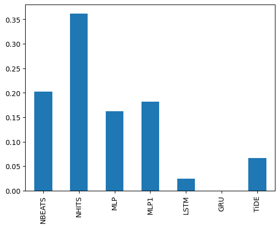
Below are the weights of each model (equal across all unique ids because weight_by_uid=False)
[13]:
ensemble.uid_coefficient['M1000'].plot.bar()
[13]:
<Axes: >
Then, we refit the neural networks are get the test forecasts
[ ]:
%%capture

nf.fit(df=train_df)
[ ]:
%%capture

fcst = nf.predict(step_size=1)
[16]:
fcst.query('unique_id=="M1"')
[16]:
| ds | NBEATS | NHITS | MLP | MLP1 | LSTM | GRU | TiDE | |
|---|---|---|---|---|---|---|---|---|
| unique_id | ||||||||
| M1 | 1994-09-30 | 2820.708008 | 2837.058838 | 2383.298828 | 2454.077393 | 2507.238525 | 2390.672607 | 2070.891602 |
| M1 | 1994-10-31 | 2353.479248 | 2515.124512 | 2158.801270 | 2129.693848 | 2583.255859 | 2305.683838 | 2451.634033 |
| M1 | 1994-11-30 | 2303.218750 | 2391.572754 | 2291.510254 | 2139.453857 | 2939.735107 | 2787.014160 | 1721.748047 |
| M1 | 1994-12-31 | 2779.379883 | 2526.065918 | 2591.097412 | 2590.750244 | 2814.711182 | 2776.601318 | 2240.189941 |
| M1 | 1995-01-31 | 2188.668457 | 2063.863525 | 2234.466553 | 1887.351929 | 2838.986328 | 2785.913818 | 1796.146118 |
| M1 | 1995-02-28 | 1911.853271 | 2175.461670 | 1985.965088 | 1816.956787 | 2691.198242 | 2710.279541 | 2631.498779 |
| M1 | 1995-03-31 | 2451.522461 | 2249.096436 | 2160.844971 | 1911.716309 | 2619.605469 | 2653.789551 | 1920.423096 |
| M1 | 1995-04-30 | 1735.337402 | 1839.155762 | 1614.420044 | 1335.228027 | 2504.666992 | 2538.148926 | 2000.088135 |
| M1 | 1995-05-31 | 1939.377686 | 2237.283691 | 2295.252930 | 2200.254150 | 2474.093994 | 2538.217285 | 3073.768555 |
| M1 | 1995-06-30 | 1589.561279 | 1889.871582 | 2036.288086 | 1789.682861 | 2385.954834 | 2385.965332 | 1627.879883 |
| M1 | 1995-07-31 | 2011.243408 | 2133.244385 | 1954.133423 | 1680.693481 | 2248.914551 | 2293.520508 | 1596.402466 |
| M1 | 1995-08-31 | 2416.882568 | 2366.746582 | 2237.609131 | 2308.385254 | 2482.302979 | 2661.940918 | 1933.988281 |
[17]:
fcst_ensemble = ensemble.predict(fcst.reset_index())
[18]:
fcst[ensemble.alias] = fcst_ensemble.values

fcst.head()
[18]:
| ds | NBEATS | NHITS | MLP | MLP1 | LSTM | GRU | TiDE | MLpol | |
|---|---|---|---|---|---|---|---|---|---|
| unique_id | |||||||||
| M1 | 1994-09-30 | 2820.708008 | 2837.058838 | 2383.298828 | 2454.077393 | 2507.238525 | 2390.672607 | 2070.891602 | 2633.876117 |
| M1 | 1994-10-31 | 2353.479248 | 2515.124512 | 2158.801270 | 2129.693848 | 2583.255859 | 2305.683838 | 2451.634033 | 2346.027112 |
| M1 | 1994-11-30 | 2303.218750 | 2391.572754 | 2291.510254 | 2139.453857 | 2939.735107 | 2787.014160 | 1721.748047 | 2263.482370 |
| M1 | 1994-12-31 | 2779.379883 | 2526.065918 | 2591.097412 | 2590.750244 | 2814.711182 | 2776.601318 | 2240.189941 | 2581.755320 |
| M1 | 1995-01-31 | 2188.668457 | 2063.863525 | 2234.466553 | 1887.351929 | 2838.986328 | 2785.913818 | 1796.146118 | 2066.855810 |
4. Evaluation
Finally, we compare all approaches
[19]:
test_df = test_df.merge(fcst, on=['unique_id','ds'], how="left")
[20]:
from neuralforecast.losses.numpy import smape
from datasetsforecast.evaluation import accuracy

evaluation_df = accuracy(test_df, [smape], agg_by=['unique_id'])
evaluation_df
[20]:
| metric | unique_id | NBEATS | NHITS | MLP | MLP1 | LSTM | GRU | TiDE | MLpol | |
|---|---|---|---|---|---|---|---|---|---|---|
| 0 | smape | M1 | 0.557906 | 0.565255 | 0.534834 | 0.545832 | 0.581718 | 0.577866 | 0.542147 | 0.548903 |
| 1 | smape | M10 | 0.203316 | 0.192507 | 0.188595 | 0.183235 | 0.187489 | 0.188297 | 0.199679 | 0.192023 |
| 2 | smape | M100 | 0.092943 | 0.084622 | 0.090799 | 0.095776 | 0.118231 | 0.119362 | 0.115861 | 0.091347 |
| 3 | smape | M1000 | 0.011336 | 0.011435 | 0.013824 | 0.010244 | 0.010340 | 0.004813 | 0.006411 | 0.010227 |
| 4 | smape | M1001 | 0.019537 | 0.019699 | 0.024808 | 0.019278 | 0.015281 | 0.007963 | 0.011028 | 0.018969 |
| ... | ... | ... | ... | ... | ... | ... | ... | ... | ... | ... |
| 1423 | smape | M995 | 0.007859 | 0.005549 | 0.012240 | 0.006474 | 0.026410 | 0.007585 | 0.010029 | 0.004580 |
| 1424 | smape | M996 | 0.022319 | 0.022942 | 0.029199 | 0.026535 | 0.009965 | 0.007247 | 0.018761 | 0.024090 |
| 1425 | smape | M997 | 0.081531 | 0.080787 | 0.077392 | 0.075628 | 0.065652 | 0.060192 | 0.080346 | 0.079193 |
| 1426 | smape | M998 | 0.008090 | 0.007945 | 0.010729 | 0.010613 | 0.026844 | 0.018760 | 0.022788 | 0.008733 |
| 1427 | smape | M999 | 0.009194 | 0.009976 | 0.018110 | 0.011560 | 0.013838 | 0.008884 | 0.012119 | 0.010070 |
1428 rows × 10 columns
[21]:
evaluation_df.drop(columns=['metric','unique_id']).mean().sort_values()
[21]:
MLpol     0.126860
NBEATS    0.127429
NHITS     0.127779
MLP1      0.130285
MLP       0.130502
GRU       0.135435
TiDE      0.139523
LSTM      0.140415
dtype: float64